


Let us understand the concept of break even and cost volume profit analysis in this blog. It is an analysis to understand at which point a company will break even. The point at which the company breaks even is known as break even point.
BREAK EVEN ANALYSIS (FORMULA BASED METHOD) Example: Consider that you bought playing chips for $20 to play a game of roulette in a casino. This $20 is your cost.
After the end of round 1, there are three possible cases:
- You win the round and are rewarded with $40. This $40 is your revenue and revenue – cost = profit. ($20 in this case)
- You lose the round and gain nothing out of it. This $0 is your revenue and revenue – cost = loss. ($20 in this case)
- You neither win nor lose and simply get the invested money back i.e.$20. This situation of no profit and no loss is known as break even.
Similarly in a corporate world, consider that you decide to open a business of assembling personal computers and selling it to the consumer.
Following will be the division of cost:
- Fixed cost: Facility
- Variable cost: Labor
(There are various factors in the respective costs, we’ve just taken 1 – 2 for your understanding).
Let, F be the fixed cost, V be the variable cost and T be the total cost.
T = F + VT = F + (QC)
Where, Q is the number of PCs and C is the cost/ unit.
Let, P be the selling price of each personal computer. Hence, Total Revenue (R) is the amount received after selling all the PCs. R = QP
So, while a company manufactures and sells any product, it goes through multiple phases.
- Phase 1: Revenue < Total cost. QP < T Loss
- Phase 2: Revenue = Total cost. QP = T Break even
- Phase 3: Revenue > Total cost. QP > T Profit
Hence, the break even sales volume formula i.e., the quantity at which the company will be break even is given by: Q = Fixed cost (F)P – C
BREAK EVEN ANALYSIS (GRAPHICAL METHOD):
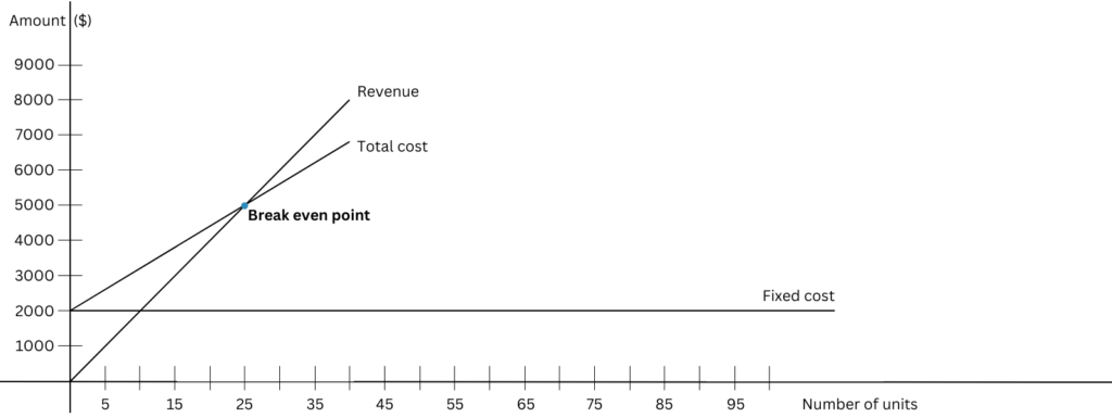
As mentioned above, we know the main components of break even analysis (fixed cost, variable cost and revenue). Fixed cost remains constant irrespective of the units sold, i.e., parallel to the x axis.
Let’s say F=$2000
For variable cost, slope of the line depends on the selling price of the unit product.
Let’s say V = $120/unit
Hence for 40 units, V = $12040 units = $4800
Therefore, T = F + QC = 2000 + 4800 = $6800
Consider the selling price P = $200/unit
Therefore, Revenue = QP = 40200 = $8000
Now comparing the equations with the standard equation of slope:
y = mx + c ——————— (1)
T = CQ + F ——————— (2)
Comparing (1) and (2),
Q is the variable (x), C is the slope (m) and F is the constant (c).
R = PQ ——————— (3)
Comparing (1) and (3),
Q is the variable (x), P is the slope (m) and F (constant) = 0.
BREAK EVEN ANALYSIS (EXPONENTIALLY GROWING BUSINESS):
Let us look at the companies that use CVP analysis. Consider a business which sells products with a continuously high demand. That business currently has 1 facility where goods are manufactured.
Let, A be the facility of production.
Let us understand the role of break even analysis in opening up another facility.
Phase 1: Let’s say 1 facility is not enough to meet the demand of products in the market. So the business (which used to run 1 shift) has now decided to run it in 2 shifts. For the 2nd (night shift), workers are demanding 1.5X times more payment. The variable cost increases but it is able to meet the demand in this case.
Phase 2: With the continuous increase in demand, even 2 shifts are not able to meet the demand. The company decides to buy new machines. The fixed cost increases in this case, but it is able to meet the demand.
Phase 3: The business is growing really well and has captured the majority of the market share. To further expand the business, it decided to start a new facility of its own.
Let, B be the new facility of production.
And again the phases will repeat in the new facility B as the demand keeps rising.
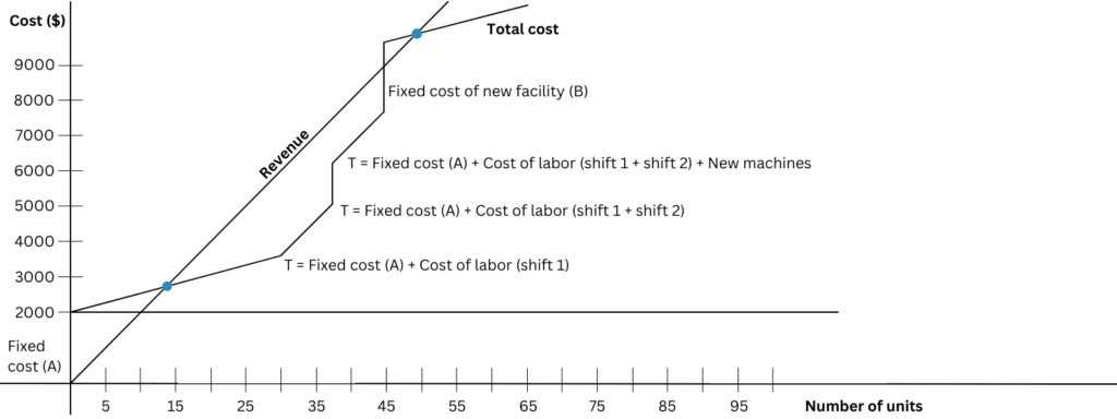
This is how growth stories of companies can be measured and defined through break even analysis.